PHYS 7B: Basic Physics II

Gravitation

Universal Law of Gravitation:

$$F_G = G \frac{m_1 m_2}{r^2}$$

where $G \approx 6.67 \times 10^{-11} \, \text{N} \cdot \text{m}^2/\text{kg}^2$ is the gravitational constant.

Gravitational Field:

$$g = \frac{F_G}{m} = G \frac{M}{r^2}$$

Satellite Motion

For a satellite in circular orbit around a planet: $F_G = \frac{mv^2}{r} = G \frac{Mm}{r^2}$ which leads to the orbital velocity: $v = \sqrt{\frac{GM}{r}}$

$a_R = \frac{v^2}{r} = \frac{GM}{r^2} = g$ is the centripetal acceleration, which is equal to the gravitational acceleration at that radius.

The period of the satellite is: $T = \frac{2\pi r}{v} = 2\pi \sqrt{\frac{r^3}{GM}}$ This is known as Kepler's Third Law.

Escape Velocity

The escape velocity from a planet is the minimum velocity needed for an object to escape the gravitational pull of the planet without further propulsion: $v_{esc} = \sqrt{\frac{2GM}{R}}$ where $R$ is the radius of the planet.

Gravitational Potential Energy

The work against gravity to move a mass $m$ from a distance $r_1$ to $r_2$ is given by: $W = \int_{r_1}^{r_2} F_G \, dr = \int_{r_1}^{r_2} G \frac{Mm}{r^2} \, dr = G Mm \left( \frac{1}{r_2} - \frac{1}{r_1} \right)$ The gravitational potential energy at a distance $r$ from a mass $M$ is, where $U(\infty) = 0$: $U(r) = -G \frac{Mm}{r}$

The negative sign indicates that the potential energy is lower (more negative) when the masses are closer together, reflecting the attractive nature of gravity. The potential energy approaches zero as $r$ approaches infinity, which means that it takes an infinite amount of energy to separate the masses completely.

Geostationary Orbits

A geostationary orbit is a circular orbit around the Earth where the satellite's orbital period matches the Earth's rotation period (24 hours). The radius of a geostationary orbit can be found using Kepler's Third Law: $T^2 = \frac{4\pi^2 R^3}{GM}$ $R^3 = \frac{GMT^2}{4\pi^2}$

Oscillations

Simple Harmonic Oscillator

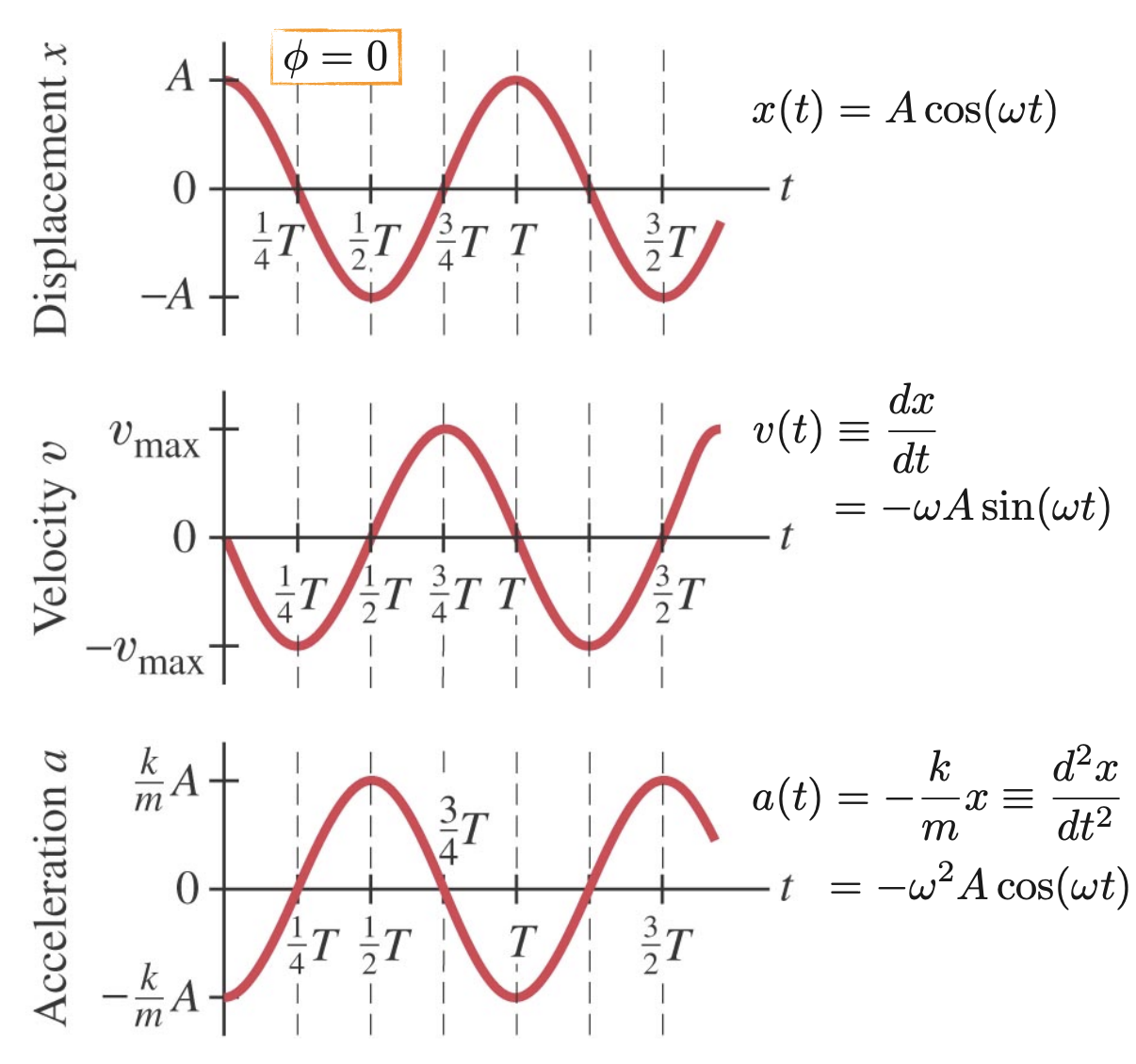
Hooke's Law: $F_s = -kx$ where $k$ is the spring constant and $x$ is the displacement from equilibrium.

$$\begin{aligned} F &= ma \\ -kx &= m \frac{d^2x}{dt^2} \\ \frac{d^2x}{dt^2} + \frac{k}{m} x &= 0 \\ \omega &= \sqrt{\frac{k}{m}} \\ \end{aligned}$$

The general solution to the equation of motion is: $x(t) = A \cos(\omega t + \phi)$ where $A$ is the amplitude, $\omega$ is the angular frequency, and $\phi$ is the phase constant determined by initial conditions.

• Period: $T = \frac{2\pi}{\omega} = 2\pi \sqrt{\frac{m}{k}}$.
• The total energy of the system is conserved and given by: $E = \frac{1}{2}mv^2 + \frac{1}{2}kx^2 = \frac{1}{2}kA^2$ Thus, $x^2 + \left( \frac{v}{\omega} \right)^2 = A^2$.

$\phi = \arctan\left( -\frac{v_0}{\omega x_0} \right)$.

Simple Pendulum

For small angles ($\theta \approx \sin \theta$):

$$\begin{aligned} F_\theta &= ma_\theta \\ -mg \sin \theta &= mL\alpha \\ -mg \sin \theta &= mL \frac{d^2\theta}{dt^2} \\ \frac{d^2\theta}{dt^2} + \frac{g}{L} \theta &= 0 \\ \omega &= \sqrt{\frac{g}{L}} \\ \end{aligned}$$

where $L$ is the length of the pendulum and $g$ is the acceleration due to gravity.

The period is: $T = 2\pi \sqrt{\frac{L}{g}}$

Physical Pendulum

For a physical pendulum, the moment of inertia $I$ and the distance $d$ from the pivot to the center of mass are used:

$$\begin{aligned} \tau &= I \alpha \\ -mgd \sin \theta &= I \frac{d^2\theta}{dt^2} \\ \frac{d^2\theta}{dt^2} + \frac{mgd}{I} \theta &= 0 \\ \omega &= \sqrt{\frac{mgd}{I}} \\ \end{aligned}$$

The period is: $T = 2\pi \sqrt{\frac{I}{mgd}}$

Wave Motion

Mechanical waves: disturbances that propagate through a medium, transferring energy without transferring matter.

Longitudinal waves: particles of the medium oscillate parallel to the direction of wave propagation (e.g., sound waves).
Transverse waves: particles of the medium oscillate perpendicular to the direction of wave propagation (e.g., waves on a string).

Sinusoidal Wave

• Crest: the highest point of the wave.
• Trough: the lowest point of the wave.
• Amplitude ($A$): the maximum displacement of the wave from its equilibrium position. (the height of the crest or trough)
• Wavelength ($\lambda$): the distance between two consecutive crests or troughs.
• Frequency ($f$): the number of oscillations per unit time.
• Period ($T$): the time it takes for one complete oscillation, $T = \frac{1}{f}$.
• Angular frequency ($\omega$): the temporal frequency of the wave, $\omega = 2\pi f = \frac{2\pi}{T}$.
• Wave speed ($v$): the speed at which the wave propagates through the medium, $v = \lambda f = \frac{\lambda}{T} = \frac{\omega}{k}$.
• Wave number ($k$): the spatial frequency, $k = \frac{2\pi}{\lambda} = \frac{\omega}{v}$.

Snapshot $y(x) = A \sin(kx + \phi)$

Traveling wave $y(x, t) = A \sin(kx - \omega t + \phi)$

Classical Wave Equation

$\frac{\partial^2 y}{\partial x^2} = \frac{1}{v^2} \frac{\partial^2 y}{\partial t^2}$ $y$ is the wave function, $x$ is the spatial coordinate, $t$ is time, and $v$ is the wave speed. The left-hand side represents the spatial curvature of the wave, while the right-hand side represents the temporal curvature.

Transverse Waves on a String

The wave speed on a string is given by: $v = \sqrt{\frac{F}{\mu}}$ where $F$ is the tension force in the string and $\mu = \frac{dm}{dx}$ is the linear mass density. $v = \lambda f = \frac{\lambda}{T}$

Coexisting Waves

Principle of superposition: when two or more waves overlap, the resulting wave is the sum of the individual waves.

• Constructive interference: when waves are in phase, their amplitudes add up, resulting in a larger amplitude.
• Destructive interference: when waves are out of phase, their amplitudes subtract, resulting in a smaller amplitude or complete cancellation.

Wave Boundary

• Fixed boundary: the wave is reflected and inverted (phase change of $\pi$).
• Free boundary: the wave is reflected without inversion (no phase change).

Standing Waves

• Incident wave: $y_i(x, t) = A \cos(kx - \omega t)$
• Reflected wave: $y_r(x, t) = -A \cos(kx + \omega t)$

Resulting wave: $y(x, t) = 2A \sin(kx) \sin(\omega t)$

$2A \sin(kx)$ is the amplitude of the standing wave, which varies with position $x$. The time-dependent part $\sin(\omega t)$ oscillates between -1 and 1, but the spatial part determines where the nodes and antinodes are located.

• Nodes: points where the amplitude is always zero (destructive interference).
• Antinodes: points where the amplitude is maximum (constructive interference). The distance between adjacent nodes or antinodes is $\frac{\lambda}{2}$, and the distance between a node and the nearest antinode is $\frac{\lambda}{4}$.

Vibrating String

Fundamental Mode: $n=1$, $\lambda_1 = 2L$, $f_1 = \frac{v}{2L}$

For a string fixed at both ends, the allowed wavelengths are: $\lambda_n = \frac{2L}{n}$ where $L$ is the length of the string and $n$ is a positive integer (the mode number). The corresponding frequencies are: $f_n = \frac{v}{\lambda_n} = \frac{n v}{2L}$ where $v$ is the wave speed on the string. The fundamental frequency (first harmonic) corresponds to $n=1$, the second harmonic corresponds to $n=2$, and so on. Each mode of vibration produces a standing wave pattern with $n-1$ nodes between the fixed ends.

$$\begin{aligned} y_n(x, t) &= 2A_n \sin\left( k_n x \right) \sin(\omega_n t) \\ k_n &= \frac{n \pi}{L} \\ \omega_n &= 2\pi f_n = \frac{n \pi v}{L} \end{aligned}$$

Sound Waves

Sound waves are longitudinal waves that propagate through a medium by compressing and rarefying the particles of the medium.

$$y(x, t) = A \cos(kx - \omega t + \phi) \\ p(x, t) = p_{max} \sin(kx - \omega t + \phi)$$

$v = \frac{\text{restoring force}}{\text{inertia}}$

In air, $v \approx 340 \, \text{m/s}$, in water $v \approx 1500 \, \text{m/s}$, and in steel $v \approx 5000 \, \text{m/s}$.

Standing Sound Waves in a Pipe

• Open at both ends: $\lambda_n = \frac{2L}{n}$, $f_n = \frac{n v}{2L}$, $n=1, 2, 3, \ldots$
• Closed at one end: $\lambda_n = \frac{4L}{n}$, $f_n = \frac{n v}{4L}$, $n=1, 3, 5, \ldots$ (only odd harmonics)

Superposition: The difference in path length traveled by two waves determines the type of interference:

• Constructive interference: $\Delta L = m \lambda$ where $m$ is an integer.
• Destructive interference: $\Delta L = (m + \frac{1}{2}) \lambda$ where $m$ is an integer.

Electrostatics

• Conductors: materials that allow electrons to flow freely (e.g., metals).
• Insulators: materials that do not allow electrons to flow freely (e.g., rubber, glass).
• Semiconductors: materials that have electrical conductivity between that of conductors and insulators (e.g., silicon).

Coulomb's Law

Coulomb's Law: The electrostatic force between two point charges:

$$\vec{F_e} = k \frac{q_1 q_2}{r^2} \hat{r}$$

where $k$ is the electrostatic constant.

$$k = \frac{1}{4\pi\epsilon_0} \approx 8.99 \times 10^9 \, \text{N} \cdot \text{m}^2/\text{C}^2 \\ \epsilon_0 \approx 8.854 \times 10^{-12} \, \text{C}^2/\text{N} \cdot \text{m}^2 \\ e \approx 1.602 \times 10^{-19} \, \text{C}$$

• attractive if the charges have opposite signs
• repulsive if they have the same sign.

Electric Field

The electric field $\vec{E}$ at a point in space is defined as the force $\vec{F}$ experienced by a positive test charge $q$ placed at that point, divided by the magnitude of the test charge:

$$\vec{E} = \frac{\vec{F}}{q}$$

The electric field due to a point charge $Q$ at a distance $r$ is given by:

$$\vec{E} = k \frac{Q}{r^2} \hat{r}$$

Continuous charge distribution

$$\vec{E} = k \int \frac{dq}{r^2} \hat{r}$$

1. Line charge distribution: $dq = \lambda dx$, $\vec{E} = \frac{2k\lambda}{r} \hat{r}$ where $r$ is the distance from the line charge to the point.
   • $\vec{E} = \int \frac{k dq}{r^2} \hat{r} = k \lambda \int \frac{dx}{r^2} \hat{r} = 2k\lambda \int_0^\infty \frac{dx}{x^2 + r^2} \hat{r} = 2k\lambda \left[ \frac{x}{r^2 \sqrt{x^2 + r^2}} \right]_0^\infty = 2k\lambda \frac{1}{r} \hat{r}$.
2. Ring charge distribution: $dq = \lambda dl$, $\vec{E} = \frac{kxQ}{(x^2 + R^2)^{3/2}} \hat{x}$ where $R$ is the radius of the ring and $x$ is the distance from the center of the ring along the axis perpendicular to the plane of the ring.
3. Disk charge distribution: $dq = \sigma dA = \sigma 2\pi r dr$, $\vec{E} = \frac{\sigma}{2\epsilon_0} \left(1 - \frac{x}{\sqrt{x^2 + R^2}} \right) \hat{x}$ where $R$ is the radius of the disk.
   • $\vec{E} = \int \frac{kx dq}{(x^2 + r^2)^{3/2}} = kx \sigma 2\pi \int_0^R \frac{r}{(x^2 + r^2)^{3/2}} dr = 2\pi k \sigma \left(1 - \frac{x}{\sqrt{x^2 + R^2}} \right) \hat{x} = \frac{\sigma}{2\epsilon_0} \left(1 - \frac{x}{\sqrt{x^2 + R^2}} \right) \hat{x}$
   • For $R \gg x$, $\vec{E} \approx \frac{\sigma}{2\epsilon_0} \hat{x}$ (infinite plane approximation).
4. Surface charge distribution: $dq = \sigma dA$, $\vec{E} = \frac{\sigma}{2\epsilon_0} \hat{n}$
   • $\vec{E} = \int \frac{k dq}{r^2} \hat{r} = k \sigma \int \frac{dA}{r^2} \hat{n} = k \sigma 4\pi \hat{n} = \frac{\sigma}{2\epsilon_0} \hat{n}$ where $\hat{n}$ is the unit normal vector to the surface.
5. Volume charge distribution: $dq = \rho dV$, $\vec{E} = \frac{\rho}{3\epsilon_0} \hat{r}$

Field Lines

• The direction of the electric field at any point is tangent to the field line at that point.
• The magnitude of the electric field is proportional to the density of the field lines: the closer the field lines are to each other, the stronger the electric field at that point.
• Field lines begin on positive charges and end on negative charges.
• Field lines never cross each other.

Electric Dipole

An electric dipole consists of two equal and opposite charges separated by a distance $d$. The dipole moment $\vec{p}$ is defined as:

$$\vec{p} = q \vec{d}$$

Direction: from the negative charge to the positive charge.

Torque $\vec{\tau} = \vec{p} \times \vec{E}$

Potential energy $U = -\vec{p} \cdot \vec{E}$

Electric Flux

The electric flux $\Phi_E$ through a surface is defined as the total electric field passing through that surface: $\Phi_E = E_\perp A = EA \cos \phi = \vec{E} \cdot \vec{A}$ $\Phi_E = \int \vec{E} \cdot d\vec{A}$ where $E_\perp$ is the component of the electric field perpendicular to the surface, $A$ is the area of the surface, and $\phi$ is the angle between the electric field and the normal to the surface.

Gauss's Law

$\Phi_E = \oint \vec{E} \cdot d\vec{A} = \frac{Q_{enc}}{\epsilon_0}$ where $Q_{enc}$ is the total charge enclosed within the Gaussian surface.

For a point charge $Q$ at the center of a spherical Gaussian surface of radius $r$: $\Phi_E = E \cdot 4\pi r^2 = \frac{Q}{\epsilon_0} \implies E = k \frac{Q}{r^2}$

For a charged insulating sphere with total charge $Q$ and radius $R$:

• For $r < R$: $Q_{enc} = \frac{Qr^3}{R^3}$, $E = k \frac{Qr}{R^3} = \frac{1}{4\pi\epsilon_0} \frac{Qr}{R^3}$
• For $r \geq R$: $Q_{enc} = Q$, $E = k \frac{Q}{r^2} = \frac{1}{4\pi\epsilon_0} \frac{Q}{r^2}$

For a charged conducting sphere with total charge $Q$ and radius $R$:

• For $r < R$: $Q_{enc} = 0$, $E = 0$
• For $r \geq R$: $Q_{enc} = Q$, $E = k \frac{Q}{r^2} = \frac{1}{4\pi\epsilon_0} \frac{Q}{r^2}$

Electric Potential Energy

$$W_{e, a\to b} = \int_a^b \vec{F}_{e} \cdot d\vec{r} = k \int_a^b \frac{q q_0}{r^2} dr = k q q_0 \left( \frac{1}{r_a} - \frac{1}{r_b} \right)$$ $$\Delta U = U_b - U_a = -W_{e, a\to b} = k q q_0 \left( \frac{1}{r_b} - \frac{1}{r_a} \right)$$ $$U = k \frac{q_1 q_2}{r}$$

Electric Potential

$$V = \frac{U}{q} = k \frac{Q}{r} = Ed$$

where $1 \, \text{V (volt)} = 1 \, \text{J/C}$.

Voltage: $V_{ba} = V_b - V_a = \frac{\Delta U}{q} = -\int_a^b \vec{E} \cdot d\vec{r}$

Multiple point charge sources: $V = k \sum \frac{q_i}{r_i}$.
Continuous charge distribution: $V = k \int \frac{dq}{r}$.

For a charged conducting sphere

• outside the sphere, the potential is the same as if all the charge were concentrated at the center
• inside the sphere, the potential is constant and equal to the potential at the surface.

For a charged insulating sphere

• outside the sphere, the potential is the same as if all the charge were concentrated at the center
• inside the sphere, the potential is given by $V = k \frac{Q}{2R^3} (3R^2 - r^2)$.

Electric field lines point from higher potential to lower potential.

Capacitance

Capacitor: two conductors separated by an insulating material (air).
Capacitance is the ability to store electrical charge.

$$C = \frac{Q}{V} = \frac{Q}{E d} = \frac{\epsilon_0 A}{d}$$

units: $1 \, \text{F (farad)} = 1 \, \text{C/V}$.

Spherical capacitor: $C = 4\pi \epsilon_0 \frac{r_a r_b}{r_b - r_a}$ where $r_a$ and $r_b$ are the radii of the inner and outer spheres, respectively.

• Capacitors in series: $\frac{1}{C_{eq}} = \sum \frac{1}{C_i}$ (same charge)
• Capacitors in parallel: $C_{eq} = \sum C_i$ (same voltage)

Energy stored in a capacitor:

$$U = \int_0^Q V \, dQ = \frac{1}{2} CV^2 = \frac{1}{2} QV = \frac{1}{2} \frac{Q^2}{C}$$

Energy density in an electric field:

$$u = \frac{U}{Ad} = \frac{1}{2} \epsilon_0 E^2$$

Dielectrics

When the capacitor is filled with a dielectric material, the capacitance increases by a factor of the dielectric constant $\kappa$: $C' = \kappa C$ $E' = \frac{E}{\kappa}$ $V' = \frac{V}{\kappa}$

Electric Circuits

Electric Current

Electric current $I$ is the rate of flow of electric charge:

$$I = \frac{dQ}{dt} = nqAv_d$$

where $n$ is the number of charge carriers per unit volume, $q$ is the charge of each carrier, $A$ is the cross-sectional area of the conductor, and $v_d$ is the drift velocity of the charge carriers.
units: $1 \, \text{A (ampere)} = 1 \,\text{C/s}$.

• Conventional current: positive charges would move, which is opposite to the actual flow of electrons.
• Real current: the actual flow of electrons, from the negative terminal to the positive terminal.

Resistance

Ohm's Law:

$$R = \frac{V}{I} = \frac{\rho L}{A}$$

where $\rho$ is the resistivity of the material, $L$ is the length of the conductor, and $A$ is the cross-sectional area.
units: $1 \, \Omega (\text{ohm}) = 1 \, \text{V/A}$.

Resistivity of metals:

$$\rho = \frac{E}{J}$$

where $E$ is the electric field and $J$ is the current density.

• Resistors in series: $R_{eq} = \sum R_i$ (same current)
• Resistors in parallel: $\frac{1}{R_{eq}} = \sum \frac{1}{R_i}$ (same voltage)

Battery

Battery: a device that converts chemical energy into electrical energy, providing a potential difference (voltage) to drive current through a circuit.

Electromotive force (emf) $\mathcal{E}$: the maximum potential difference provided by the battery when no current is flowing.
Internal resistance $r$: the resistance within the battery that causes a voltage drop when current flows.
Terminal voltage $V$: the actual voltage across the battery terminals when current is flowing, given by

$$V = \mathcal{E} - Ir$$

Power

Power delivered by the battery:

$$P = IV = I(\mathcal{E} - Ir) = I\mathcal{E} - I^2 r$$

Power delivered to the resistor:

$$P_R = IV = I^2 R = \frac{V^2}{R}$$

The first term $I\mathcal{E}$ represents the power supplied by the battery, while the second term $I^2 r$ represents the power lost due to the internal resistance of the battery. The efficiency of the battery can be calculated as $\text{Efficiency} = \frac{P_{\text{useful}}}{P_{\text{total}}} = \frac{I\mathcal{E} - I^2 r}{I\mathcal{E}} = 1 - \frac{Ir}{\mathcal{E}}$

Kirchhoff's Laws

• Kirchhoff's Current Law (KCL): The total current entering a junction equals the total current leaving the junction.
• Kirchhoff's Voltage Law (KVL): The sum of the potential differences around any closed loop in a circuit must equal zero.

RC (Resistor-Capacitor) Circuits

Equations:

$$\begin{aligned} \sum V = 0 &\Rightarrow \mathcal{E} - iR - \frac{q}{C} = 0 \\ i = \frac{dq}{dt} &\Rightarrow \frac{dq}{dt} = \frac{\mathcal{E}}{R} - \frac{q}{RC} \\ \frac{dq}{dt} &= \frac{q - \mathcal{E}C}{-RC} \\ \int_0^Q \frac{dq}{q - \mathcal{E}C} &= -\int_0^t \frac{dt}{RC} \\ \ln \left| \frac{q - \mathcal{E}C}{-\mathcal{E}C} \right| &= -\frac{t}{RC} \\ \end{aligned}$$

When a capacitor is charging through a resistor:

$$\begin{aligned} Q(t) &= C \mathcal{E} \left(1 - e^{-\frac{t}{RC}} \right) \\ V(t) &= \mathcal{E} \left(1 - e^{-\frac{t}{RC}} \right) \\ I(t) &= \frac{\mathcal{E}}{R} e^{-\frac{t}{RC}} \\ \end{aligned}$$

Charge increases in a characteristic time scale where time constant is $\tau = RC$.

When a capacitor is discharging through a resistor:

$$\begin{aligned} Q(t) &= Q_0 e^{-\frac{t}{RC}} \\ V(t) &= V_0 e^{-\frac{t}{RC}} \\ I(t) &= -\frac{V_0}{R} e^{-\frac{t}{RC}} \\ \end{aligned}$$